Detailed analysis#
automea also allows the user to perform a custom and detailed analysis of MEA datasets.
The methods from the Analysis() class that are used in the analyze_dataset() function can also be accessed directly.
Load signal from dataset#
For instance, let’s say we want to analyze a specific dataset, we can inform its location changing the path_to_dataset attribute, and load it by using the loadh5() method - this can take some time depending on the dataset size and your processor.
import automea
am = automea.Analysis()
am.path_to_dataset = '../../qneuron/mea-reproduce-results/mea-h5-datafiles/'
am.loadh5('AH22C001_3039_DIV14.h5')
After the file is loaded, we have a signal attributed already loaded, containing the signal for all wells/channels in the dataset
am.signal
array([ 6, -6, 7, ..., 5, -10, 14], dtype=int32)
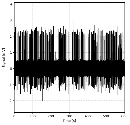
The units of this signal look a bit off compared to usual values from MEA measurements. This is because the data is saved as an integer array to facilitate its use in some calculations, but can be converted to mV by using the class method convert_signal() and the conversion parameters obtained from the dataset and saved as attributes.
signal_in_mV = am.convert_signal(am.signal[0], am.adZero, am.conversionFactor, am.exponent)
am.plot_window(signal_in_mV, yunits = 'mV')
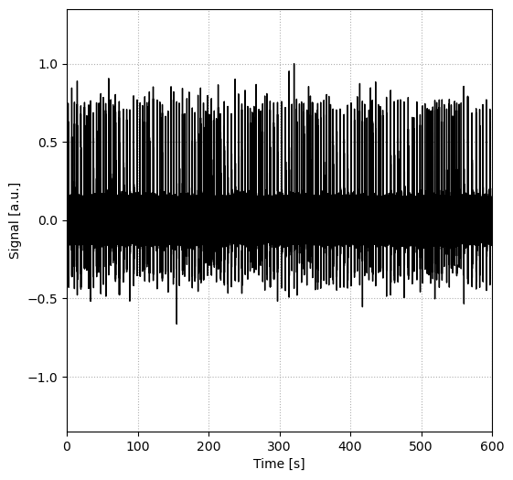
Alternatively, a normalized signal can be used, for which the signal is always between -1 and 1 normalized for every channel. This is used in the machine learning models to detect bursts for example. We can get a normalized signal by using the dedicated method:
signal_norm = am.normalize_signal(am.signal[0])
am.plot_window(signal_norm, yunits = 'a.u.')
Detect threshold, spikes, and bursts#
From the loaded signal we can detect (in order) threshold, spikes, reverberations, and bursts, by using the designated class methods.
To speed up the process, let’s use only the first-channel signal from the dataset. We can reduce our signal attribute by using a method named loadsignal().
am.loadsignal(am.signal[0])
am.signal
array([ 6, -6, 7, ..., 5, -10, 14], dtype=int32)
We can see the signal attribute is now a one dimensional array. This method can also be used by loading any array as the signal, circumventing the restriction of using a specific data file - like the dataset we loaded before, which had a very specific structure.
The threshold can be obtained by doing:
am.detect_threshold()
which populates the threshold attribute with an array.
am.threshold
array([172.04914396])
In this case we have one threshold, since we have only one signal.
The value of threshold comes from the integer signal array, not holding any unit value whatsoever. Similar to what we did for the signal, we can get a threshold value in mV, or a normalized threshold.
threshold_in_mV = am.convert_threshold(am.threshold, am.adZero, am.conversionFactor, am.exponent)
threshold_in_mV
array([10.25481718])
threshold_norm = am.normalize_threshold(am.signal, am.threshold)
threshold_norm
array([0.20099199])
We can visualize the threshold with the signal, by passing the threshold as an argument to the plot_window() method.
am.plot_window(am.signal, threshold = am.threshold)

With the signal and the threshold, we can detect spikes using the detect_spikes() method.
am.detect_spikes()
am.spikes
The spikes attributte consists of a list with all the timestamps in which there is a spike. If signal has n > 1 channels, spikes will be a list of n-lists.
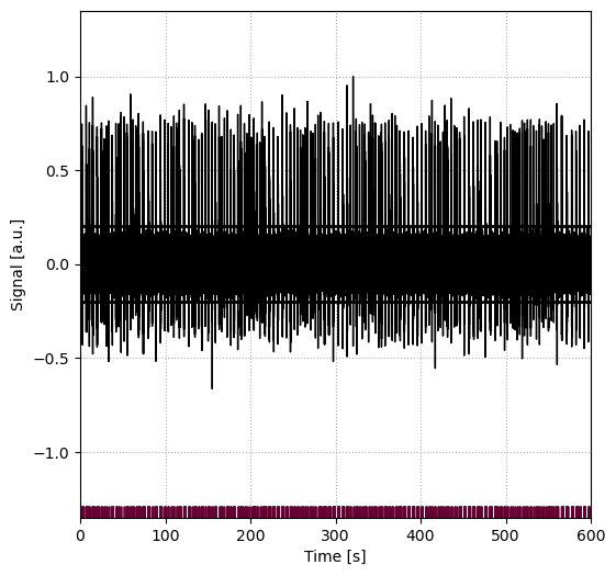
We can visualize spikes together with the signal and threshold by doing:
am.plot_window(am.signal, threshold = am.threshold, spikes = am.spikes)
Reverberations and bursts can be detected using specific methods. Here we can choose how we will detect them. The package makes use of the Max Interval Method, which parameters can be set manully, using a pre-defined default set of values, or by predicting optimal values with a machine learning model.
This choice is made by passing an argument to the detect…() methods. For instance, if we want the signal30 model to detect reverbeations, we first load it
am.model_name = 'signal30.h5'
am.loadmodel()
and tell the method we want to perform a detection using the model method.
am.detect_reverbs(method = 'model')
am.reverbs
The same can be done for bursts and network bursts - in the case with multiple channels.
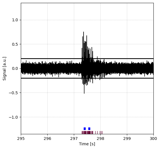
We can now visualize the signal accompanied by spikes and reverberations. It’s possible to choose specific start and end times, to analyze the reverberations in detail.
am.plot_window(am.signal,threshold = am.threshold, spikes = am.spikes, reverberations = am.reverbs)
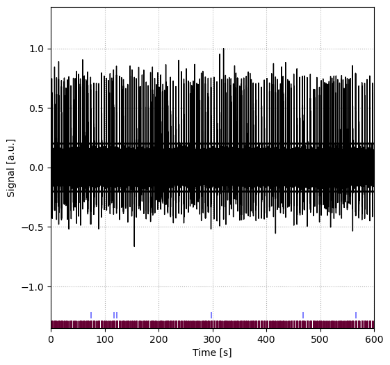
am.plot_window(am.signal,start_time = 295, duration = 5, threshold = am.threshold, spikes = am.spikes, reverberations = am.reverbs)